Support Vector Machines explained

Published Nov 26, 2022

Disclaimer: this does not aim to fully cover the possibilities of SVM models. It merely describes the basic concepts related to them. Some details are skipped on purpose with the intention of keeping it short.

You can find a from scratch implementation of an SVM in Julia here: https://github.com/shilangyu/SVM-from-scratch

Invented by Vladimir Vapnik. SVM is a binary linear classifier for supervised learning (though, can be used for regression as well). Input data are points in Euclidean space.

Let $D = {(x_{i}, y_{i}) : i \in {1, \dots, n}}$ be a dataset which is a set of pairs where $x_{i} \in R^{d}$ is a data point in some $d$ -dimensional space and $y_{i} \in {- 1, 1}$ is a label of the appropriate $x_{i}$ data point classifying it to one of the two classes. The model is trained on $D$ after which it is present with $x_{i + 1}$ and is asked to predict the label of this previously unseen data point.

The prediction function will be denoted by $p : R^{d} \to {- 1, 1}$ . The output of a prediction will be denoted by $\overset{y}{^}$ . SVM is a description of such a model and how can one optimize $p$ given a dataset and a loss function.

SVM’s goal is to construct a prediction function which will represent a hyperplane that can be used to divide the space into two parts. One SVM model is considered to be better than a different SVM model for the same dataset if the margin (distance) between the hyperplane and the nearest data point is maximized. The nearest data point to the hyperplane is called the support vector. Therefore we have a clear metric to optimize.

Recall the general equation of a hyperplane: $w \cdot x - b = 0$ where $w \in R^{d}$ denotes a normal vector to the hyperplane and $b \in R$ is the offset ( $\frac{b}{∣∣ w ∣∣}$ determines the offset from the origin along the normal vector $w$ ). Since our goal is the find the optimal hyperplane, we end up with $d + 1$ trainable parameters ( $∣ w ∣ + 1$ ). Once the hyperplane is found we can construct two additional parallel hyperplanes which reside at the support vectors of the two classes, $w \cdot x - b = - 1$ and $w \cdot x - b = 1$ . Then, all points from the dataset adhere to the following

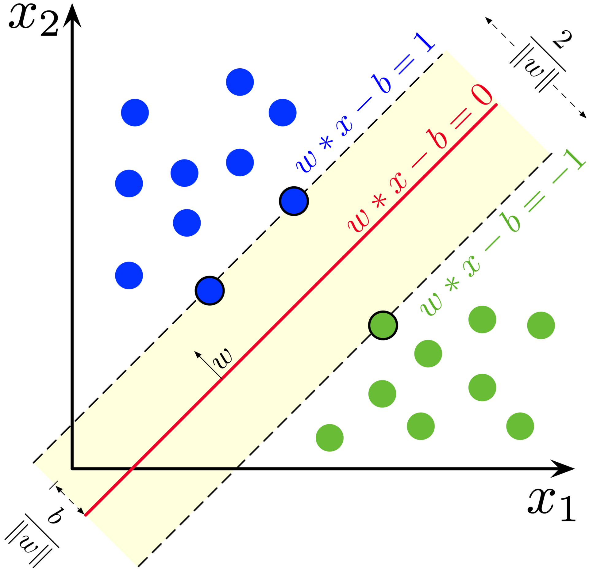
y_{i} = {- 1 1 if w \cdot x_{i} - b \leq - 1 if w \cdot x_{i} - b \geq 1 ⟹ y_{i} (w \cdot x - b) \geq 1

Since $\frac{1}{∣∣ w ∣∣}$ is the margin and we want to maximize it, the problem can be restated as a minimization problem of $∣∣ w ∣∣$ . Our predictor can be neatly expressed as $p (x) = sign (w \cdot x - b)$ with an edge case of when $x$ lies perfectly on the hyperplane, then we can just assume that $p (x) = 0$ belongs to one of the two classes. This is called a hard-margin SVM since it works only for perfect datasets which do not have outliers.

Now that we have the model we need to introduce a way to train it. There are many techniques to do so. Here we will focus on one which uses gradient descent. Firstly, we need some function we want to optimize. We will use the hinge function which will suit our needs well: $H (x_{i}, y_{i}) = max (0, 1 - y_{i} (w \cdot x_{i} - b))$ . Notice, that when the guess is correct, then $y_{i} (w \cdot x_{i} - b) \geq 1$ as shown before, thus $H = 0$ . If the guess is incorrect, $H \geq 0$ . So if for every data point $H = 0$ then we have found a hyperplane that divides the space correctly. Hinge loss introduces a soft-margin since it allows for misclassification with a quantifiable result. We also have to incorporate the minimization of $∣∣ w ∣∣$ as previously stated. Finally, we can define a loss function over the whole dataset which we will want to minimize:

ℓ (w, b) = λ ∣∣ w ∣ ∣^{2} + \frac{1}{n} i = 1 \sum n H (x_{i}, y_{i}) = λ w \cdot w + \frac{1}{n} i = 1 \sum n max (0, 1 - y_{i} (w \cdot x_{i} - b))

Here $λ > 0$ is the regularization hyperparameter controlling the trade-off between correct predictions and large margins. To perform gradient descent we will need to compute the partial derivatives with respect to the trainable parameters ( $w$ and $b$ ). Sadly the hinge function is not differentiable, but we can consider it by splitting it into two cases: when we reach the left and right case of the $max$ function.

H (x_{i}, y_{i}) = {0 1 - y_{i} (w \cdot x_{i} - b) if y_{i} (w \cdot x_{i} - b) \geq 1 otherwise

Which yields the following gradient (recall that $w$ is a vector):

\nabla ℓ = \frac{\partial ℓ}{\partial w} \frac{\partial ℓ}{\partial b} = 2 λ w + \frac{1}{n} \sum_{i = 0}^{n} {0 - y_{i} x_{i} if y_{i} (w \cdot x_{i} - b) \geq 1 otherwise \frac{1}{n} \sum_{i = 0}^{n} {0 y_{i} if y_{i} (w \cdot x_{i} - b) \geq 1 otherwise = 0

For each training example from our dataset we can now first check the $y_{i} (w \cdot x_{i} - b) \geq 1$ condition. We can perform gradient descent with the gradient specified above and conditionally apply a different gradient based on the condition. Since the gradient points to the steepest ascent and our task is to minimize the function, we will subtract the gradient instead of adding it. Our parameters will now converge iteratively, where $k$ is the iteration number for each $i$ :

w_{k + 1} = {w_{k} - 2 λ w_{k} w_{k} - (2 λ w_{k} - y_{i} x_{i}) = w_{k} - 2 λ w_{k} + y_{i} x_{i} if y_{i} (w_{k} \cdot x_{i} - b) \geq 1 otherwise

b_{k + 1} = {b_{k} b_{k} - y_{i} if y_{i} (w \cdot x_{i} - b_{k}) \geq 1 otherwise

See linear_soft_margin_svm.jl for a practical implementation of the so far introduced concepts

So far we have been generating hyperplanes which intrinsically suffer from being able to classify only linearly separable datasets. For instance, the XOR function is not linearly separable. To solve non-linear problems one has to introduce non-linearity to the model, similarly to how neural networks use non-linear activation functions. One such way would be to introduce extra dimensions where the dataset can be divided by a hyperplane. If $R^{d}$ is the space of the data points, we want to find such a mapping, called feature map, $φ : R^{d} \to R^{r}$ for some $r \in N$ (preferably $d < r$ since we want to increase the dimensionality) together with a kernel function $k : R^{d} \times R^{d} \to R$

k (x, y) = ⟨ φ (x), φ (y)⟩

Since we are operating in the euclidean space with the dot product as the inner product space, we can rewrite $k$ as $k (x, y) = φ (x) \cdot φ (y)$ . Direct computation of $φ$ is not needed, we will only need to find the kernel function. This kernel function will replace dot products used throughout the SVM method.

Note that if we set $φ = id$ then $k (x, y) = ⟨ φ (x), φ (y)⟩ = ⟨ x, y ⟩ = x \cdot y$ , which gives us the SVM for linearly separable problems. Now, this problem can be expressed as a primal one and proceed with gradient descent as we did for the linear case. However, for some not precisely known reason the literature about SVMs has converged towards solving it as a Lagrangian dual and, as O. Chapelle (2007) argues, the primal one can provide many advantages. In both the primal and dual problem formulation $φ$ is never directly computed, it is always used indirectly through the kernel function. So, to not diverge from literature I will present the dual problem which requires Quadratic Optimization instead of gradient descent.

To start we introduce the Lagrange primal which we want to minimize on $w$ and $b$

L_{1} (w, b, α) = λ \frac{1}{2} ∣∣ w ∣ ∣^{2} - i = 1 \sum n α_{i} (y_{i} (w^{T} φ (x_{i}) - b) - 1)

subject to $α_{i} \geq 0$ . This is not enough since we want to get rid of the $φ$ . Thus we attempt to minimize on $w$ and $b$ to derive the dual:

\frac{\partial L _{1}}{\partial w} = 0 = λ w - i = 1 \sum n α_{i} y_{i} φ (x_{i}) ⟹ w = i = 1 \sum n α_{i} y_{i} φ (x_{i})

\frac{\partial L _{1}}{\partial b} = 0 = - i = 1 \sum n α_{i} y_{i} ⟹ i = 1 \sum n α_{i} y_{i} = 0

Which yields the dual which has to be minimized as

L_{2} (α) = \frac{1}{2} i = 1 \sum n j = 1 \sum n y_{i} α_{i} φ (x_{i}) \cdot φ (x_{j}) y_{j} α_{j} - i = 1 \sum n α_{i} = \frac{1}{2} i = 1 \sum n j = 1 \sum n y_{i} α_{i} k (x_{i}, x_{j}) y_{j} α_{j} - i = 1 \sum n α_{i}

Subject to $\sum_{i = 1}^{n} α_{i} y_{i} = 0$ and $0 \leq α_{i} \leq λ^{- 1}$ . To solve this one has to use quadratic optimization which is well beyond the scope of this document. A popular approach is the SMO algorithm (J. Platt 1998).

In the new space $w$ can be expressed as the following linear combination, for $c$ support vectors (ie. those with $α_{i} > 0$ ):

w = j = 1 \sum c α_{j} y_{j} φ (x_{j})

And $b$ can be computed from the support vectors as well:

b = \frac{1}{n} i = 1 \sum n w \cdot φ (x_{i}) - y_{i} = \frac{1}{n} i = 1 \sum n j = 1 \sum c α_{j} y_{j} k (x_{j}, x_{i}) - y_{i}

Then we can return to our predictor function

p (x) = sign (w \cdot φ (x) - b) = sign (i = 1 \sum c α_{i} y_{i} φ (x_{i}) \cdot φ (x) - b) = sign (i = 1 \sum c α_{i} y_{i} ⟨ φ (x_{i}), φ (x)⟩ - b) = sign (i = 1 \sum c α_{i} y_{i} k (x_{i}, x) - b)

Many kernel function exist and can be used for different use cases. A common choice for a kernel function is the basis radial function, it has a single hyperparameter $γ > 0$ :

rbf (x, y) = exp (- γ ∣∣ x - y ∣ ∣^{2})

See non_linear_svm.jl for a practical implementation of a SVM with a $rbf$ kernel trained on a non linearly separable dataset.

If the amount of classes is larger than 2, we can construct multiple SVM and treat them as a single larger SVM. There are many popular techniques for that, but here two most popular approaches will be mentioned. Let there be $m$ classes.

one-versus-all: we construct $m$ SVMs trained to treat the dataset as having two classes: one for the target class, and the other for all other $m - 1$ classes. To then perform predictions, we can run the new $x_{i + 1}$ point through all $m$ SVMs and see which one is the most certain about its prediction. Note, that the definition of the prediction function had a co-domain of ${- 1, 0, 1}$ so it is not possible to decide which SVM is the most certain. Therefore the prediction function has to be altered to produce quantifiable scores.
one-versus-one: we construct $(2 m)$ SVMs for every combination of pairs of classes. Then to perform predictions, we run all SVMs and collect votes. The class with most votes wins.

In the case of one-versus-all the prediction function has to be reformulated unlike in the one-versus-one case. However, one-versus-one comes with a $(2 m) = O (m^{2})$ quadratic amount of SVMs unlike the $m = O (m)$ linear one for one-versus-all. Thus the one-versus-one approach will scale horribly for larger values of $m$ .

See multiclass_svm.jl for a practical implementation of a multiclass SVM using the one-versus-all approach.

All images taken from the well-written Wikipedia article on SVMs https://en.wikipedia.org/wiki/Support_vector_machine
V. Vapnik, Statistical Learning Theory (1998)
O. Chapelle, Training a Support Vector Machine in the Primal (2007)
J. Platt, Sequential Minimal Optimization: A Fast Algorithm for Training Support Vector Machines (1998)

Correct mistake Repository

Support Vector Machines explained

What if the problem is not linearly separable?

What if the problem isn’t binary?

References